Multi-step Route Planning

Task: Repeatedly expand single-step retrosynthesis until every leaf is a purchasable building block, thereby producing a complete synthetic route to the target molecule. SynOmega searches over a single AND-OR graph; the default algorithm is Retro* (Chen et al., ICML 2020), with MCTS and best-first offered as two interchangeable alternatives.

1. Search graph: the AND-OR graph

flowchart TD
    T["Target molecule<br/>MolNode (OR)"] --> R1["Reaction A<br/>RxnNode (AND)"]
    T --> R2["Reaction B<br/>RxnNode (AND)"]
    R1 --> M1["Reactant 1 (OR)"]
    R1 --> M2["Reactant 2 (OR)"]
    R2 --> M3["Reactant 3 (OR)"]
    M1 --> S1["✔ Purchasable"]
    M2 --> R3["Reaction C (AND)"]
    M3 --> S2["✔ Purchasable"]

• MolNode (OR node): a molecule; its multiple candidate reactions stand in an "or" relation — solving any one of them solves the molecule. A molecule is solved iff in_stock or any child reaction is solved.
• RxnNode (AND node): a reaction; its reactants stand in an "and" relation — it is solved only when all reactants are solved. Its cost is cost = -log(max(score, 1e-12)), which makes cost additive along a route.
• DAG rather than tree: molecule nodes are interned by InChIKey, so a given molecule is unique in the graph and is naturally deduplicated; add_reaction performs cycle detection (rejecting a reactant that is an ancestor, avoiding X ← X); propagate_solved propagates the solved state bottom-up by iteration (not recursion) to prevent stack overflow.

2. Default algorithm: Retro*

Retro* is a best-first AND-OR search equipped with a value function. It maintains a cost-to-go estimate for each molecule and preferentially expands the "most promising" frontier nodes:

• \( r_n(m) = 0 \) (purchasable); \( = V(m) \) (unexpanded, using the heuristic estimate); \( = \min_r \big[\, \mathrm{cost}(r) + \sum_{c} r_n(c) \,\big] \) (expanded).
• The global cost of reaching a molecule is \( V(m) = r_n(m) + \delta(m) \), where \( \delta(m) \) is the cost of "the rest of the tree that must be paid for in order to reach m" (recursing toward the root, including the sum of sibling \(r_n\)).

function retrostar(target, budget, expansion_width=50):
    graph = AndOrGraph(target)
    while not graph.root.solved and not budget.exhausted(expansions):
        frontier = select_frontier(graph)           # unsolved/unexpanded nodes, take a batch by ascending V
        if frontier is empty: break
        preds = model.predict_batch(frontier_smiles, expansion_width)
        for node, pred_list in zip(frontier, preds):
            node.expanded = True; expansions += 1
            attach_reactions(graph, node, pred_list) # create RxnNodes; mark purchasable children solved
        refresh(graph)                               # fixed-point iteration: recompute all r_n until stable
    return SearchResult(solved=graph.root.solved, graph, stats)

refresh is a bottom-up fixed-point iteration (at most 64 rounds) — because the search graph is small, recomputing everything from scratch is cheaper than a single model call, so no incremental optimization was done.

value function (supplies the heuristic \(V\))

Name	\(V(m)\)	Purpose
MolSizeValue (default)	scale·max(0, heavy_atom_count − free_atoms)	Larger molecules are farther from purchasable
ZeroValue	0 (admissible)	Retro* degenerates to uniform-cost
ConstantValue	fixed penalty per unsolved molecule	Prefers fewer unsolved molecules

3. Interchangeable algorithms: MCTS and best-first

• MCTS (mcts, Segler 2018 / AiZynthFinder style): selection (UCT descent, skipping dead nodes) → expansion + rollout (greedy playout, rollout_depth=3) → backpropagation. The reward is the fraction of purchasable molecules in the final frontier (partial credit, better than 0/1). exploration=1.4, expansion_width=25.
• best-first (bfs): a g+h priority queue (heapq), where g approximates cumulative reaction cost and h comes from the value function; with ZeroValue it is uniform-cost, and with a heuristic it approximates A*. Serves as a reference implementation.

The top-level Planner is assembled in the order base model → (optional plausibility filter) → (optional cache) → search algorithm (the filter sits inside the cache, so the cache already holds filtered expansions); Budget(max_depth=6, time_limit=60, max_expansions=500) is the default budget, tightened to a unified operating point for evaluation (see the overview).

4. Evaluation results

On the 1000-target ChEMBL set, under aligned budgets (k=10), we compare the original model against the simplification-constrained model (see the retro chapter).

4.1 Expansion-width sweep (k = 3…10)

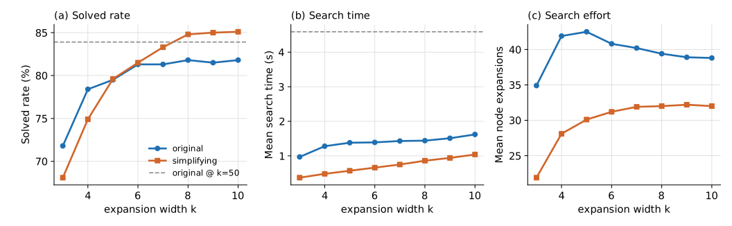
Key points: the solved rate of the simplification-constrained model climbs to 85.1% at k=10, and at k≈8 it overtakes the expensive reference of "the original model @ k=50" (83.9%); the original model plateaus at roughly 81.8%. The curves flatten around k≈6–8, and we select k=10 as the operating point.

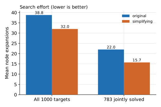
4.2 Efficiency gain from the simplification constraint (k=10)

Comparison	Original	Simplified	Change
solved rate (1000 targets)	81.8%	85.1%	+3.3 pp (McNemar p=1.5e-3)
mean expansions (all)	38.8	32.0	−18%
mean expansions (783 jointly-solved targets)	22.0	15.7	≈ −30% (Wilcoxon W=20881, p=8.6e-21)
median search time	0.49 s	0.32 s	about one-third less

That is: without any loss of coverage, the simplification constraint lowers the expansion cost of multi-step search by about 18% (nearly 30% on jointly-solved targets). This is a search-efficiency gain, NOT a "simpler = more reasonable" claim.

4.3 Comparison with AiZynthFinder

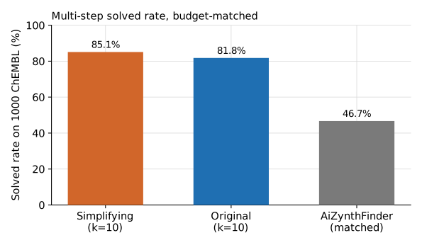
On the same 1000 ChEMBL, the same ZINC building-block set, aligned budgets (top-10 expansion, depth 5, 100 iterations), and the same GPU:

System	Search algorithm	solved	median search time
SynOmega (simplified)	Retro*	85.1%	~0.3 s
SynOmega (original)	Retro*	81.8%	~0.5 s
AiZynthFinder v4.4.1	MCTS	46.7% (467/1000)	4.1 s

SynOmega achieves roughly 1.8× the solved rate of AiZynthFinder; 391 targets are solved only by SynOmega and 7 only by AiZynthFinder; the median search time of the simplified model is about 1/13 that of AiZynthFinder.

5. Limitations

• Retro*'s refresh recomputes the whole graph, which is not optimal on very large search graphs (not a bottleneck at the current scale).
• The solved rate depends on building-block coverage and the recall of the single-step model; out-of-distribution and very large / multi-component targets remain difficult.